Network Precision | Audio-over-IP as a Signal Source for Line Array Speaker Systems

Acoustic coherence in the field of tension between waveguide mechanics and network synchronization.

v1.1.1. | 2026-04-28 | © Bodo Felusch

Switch language

Reference: Timing Precision Requirements for Line Arrays

The requirements for mechanical precision in line array loudspeakers are well-established. The waveguide is the most precision-critical component, guiding the energy of the high-frequency drivers as coherently — i.e. as phase-linearly — as possible to the acoustic aperture. The race for the optimal waveguide has largely been run out, constrained by patent law. So why not open a new front?

First, we need to establish a benchmark for the precision we are aiming for. Everything discussed below is evaluated at 20 kHz. We define the acceptable phase difference in the waveguide as 1/4 of the wavelength — i.e. a 90° phase difference — yielding a summation result of +3 dB from two coherent sound sources at 0 dBr each. For mechanical construction this translates to an acceptable tolerance window of 4.3 mm across the full operating temperature range. Coupling between adjacent elements is excluded from this discussion; sufficient literature already exists on that topic. 

An equivalent error budget at the upstream electronic level corresponds to approximately 12.5 µs of time difference between two coherent signals at exactly 0 dBr. This is slightly more than one sample period at 96 kHz, which has a duration of 10.4 µs. As a physical reference point: a temperature difference of just 1°C across 10 m causes a propagation delay difference of approximately 51 µs — exceeding the entire electronic error budget (~12.5 µs) by a factor of four. This strikingly illustrates that acoustic environmental conditions are often the limiting factor in practice, not the electronics.

New technologies such as beamforming — which aim to steer the directional behaviour of a line array segment electronically — impose far more stringent precision requirements. This is almost certainly the reason why electronically steered systems rely on fixed mechanical splay angles. When using FIR filters, the limiting factor at low frequencies is latency: at 96 kHz with 2048 taps, one must accept 10.6 ms of latency, with only 46.9 Hz of bandwidth per tap — all-pass filters can provide relief here. At high frequencies, the enclosure and drivers themselves are the limiting constraint: to accurately control phase to within 180° at 20 kHz, the physical tolerance must be kept below 8.5 mm. 

In short: at low frequencies, time is the limiting resource; at high frequencies, space is.

Fundamentals of Synchronisation

Clock Drift
Before mobile phones united us on a common time reference, free-running clocks defined our individual, absolute, yet perpetually inaccurate sense of time. Mechanically constructed timepieces and quartz watches, for instance, vary in their precision. Even two identical quartz watches will not remain in agreement over time. Assume a quartz oscillating at 32,768 Hz with a drift of ±10 ppm. If two such watches are both set to 00:00 on the 1st of January and left running, they will show different times after just a month — they drift apart. In the worst case, the two clocks diverge by 1.7 seconds per day, and by 52 seconds after one month. Anyone who has recorded picture and sound on separate devices knows that both recorders must be synchronised to maintain lip sync throughout the recording. The problem is exactly the same as with the two quartz watches: neither is locked to a common reference. Clock drift is a frequency offset — a mistuning of the rate at which the clock oscillator is supposed to run.

Interface Jitter
When two digital audio devices are operated at the same sample rate, connected digitally in series, but each locked to its own internal clock, the same problem recurs — they drift apart and audible clicks begin to appear. A Clock Leader must be defined, and all digitally connected devices must be synchronised to it as Clock Followers. In this process, the clock signal is transmitted over a physical medium, giving rise to Interface Jitter between the digital interfaces. In serial (daisy-chain) cabling, this interface jitter accumulates and corrupts the clock signal. To put it concisely: the clock edges smear in time, and the receiver can no longer reliably distinguish between a one and a zero. The underlying causes are cable-induced errors such as impedance mismatch, capacitance, reflections, excessive cable length, or simply physical damage and ageing. Star-topology wiring helps to keep interface jitter low. A clock signal corrupted by interface jitter can be regenerated through re-clocking: the signal is buffered and re-generated by an internal clock that is itself synchronised to the Clock Leader.

Clock Wander & Clock Jitter
Beyond the fundamental long-term drift that every oscillator exhibits — no matter how precise — there are also short-term fluctuations. Imagine listening to a motivating mixtape through headphones, running for 30 minutes, fully in the groove. Then you sneeze, stumble, momentarily lose the beat — but a few seconds later you are back in sync with the music. After four or five hours in the blazing summer heat, your muscles begin to tire and your step starts to drift off the beat. The same phenomenon occurs — with far smaller deviations — in every clock source. Beyond drift, there are low-frequency fluctuations in phase — phase noise — caused by environmental influences such as temperature variation, power supply instability, or mechanical stress. This low-frequency "wobble" below 10 Hz is called Clock Wander. High-frequency phase noise above 10 Hz is called Clock Jitter, and it comes in two distinct varieties. Matter is fundamentally never at rest; the purity and properties of semiconductors vary in quality. This gives rise to Random Jitter, which follows an unpredictable Gaussian distribution — almost as if matter itself were an overarching clock source, the fundamental noise floor of time. Deterministic Jitter, by contrast, is consistent and repeatable — the consequence of our own design decisions. Electronic circuits suffer from crosstalk, power supply ripple, electromagnetic interference, and impedance mismatches. Clock jitter is a "tremor" around the target frequency at which the oscillator is supposed to run.

Synchronisation Accuracy
Every digital transmission system requires a shared clock reference. The Clock Leader is the authoritative time reference for all Clock Followers, which lock to it using a PLL (Phase-Locked Loop) circuit that nudges their internal oscillator faster or slower as required. How well a system achieves this is described by its synchronisation accuracy. In Dante with PTPv1, the target synchronisation accuracy is 1 µs between a single transmitter and receiver pair, and 2 µs in multi-receiver configurations. Under degraded network conditions, a guaranteed synchronisation accuracy of one sample length is maintained.

What Time Is It — Really?
The most precise clock we know of is the atomic clock, which derives its time reference from the radiation transitions of electrons in free atoms. Caesium, rubidium, hydrogen, and more recently strontium are the most common atoms used, with a drift of approximately one second per 300 million years. While this may seem like more than enough precision to keep an appointment, it is in fact insufficient for the highly precise technology we have built. Even an atomic clock drifts by 1 nanosecond after approximately 110 days.
If we want to synchronise to 1 ns precision globally — for example, to achieve 1-metre GPS positioning accuracy — we need a more elaborate approach. We therefore average the historical measurements of some 400 atomic clocks at 60 institutions worldwide to form the International Atomic Time (TAI), from which the Coordinated Universal Time (UTC) is derived. This is, in essence, Leader Clock Number One. GPS satellites carrying their own atomic clocks, synchronised to ground stations, form Leader Clock Number Two. These two systems are not synchronised to each other; they run independently, typically diverging by no more than approximately 20 ns. UTC is not directly relevant to the rest of this discussion, but one fact is worth noting: due to the Earth's irregular rotation, leap seconds are periodically inserted to keep UTC aligned. GPS time, by contrast, has been running continuously since 1980. GPS time therefore currently runs exactly 18 seconds ahead of UTC. TAI had a 10-second head start over UTC at its launch in 1972, and a 19-second lead over GPS time at the GPS epoch of 6 January 1980 at 00:00:00 — an offset that has remained constant since. TAI and GPS both run continuously without leap seconds. As of May 2026, TAI leads UTC by 37 seconds (18 s + 19 s); this must be taken into account when converting between PTP/TAI and UTC.

Reference: GPS Jitter

The GPS system is an excellent source of high-precision, globally synchronised time information. The jitter level depends heavily on the quality of the receiver: the receiver's internal oscillator must suppress the inherent GPS jitter. Typical values range from a few nanoseconds to 50–100 ns; at the higher end, the timing is effectively derived from the receiver's own oscillator and only disciplined by GPS.

Reference: Wordclock-Jitter

The datasheet of an industry-benchmark wordclock generator provides the following specifications:

• Drift:    Clock frequency leader mode:       44.1 or 48 kHz ± 25 PPM, -5 +50 °C.
• Jitter:    Intrinsic clock jitter:   10Hz)
  
  

GPS offers lower drift; the wordclock offers lower jitter. In broadcast environments, both techniques are therefore combined.

Reference: Jitter Perception Threshold in Digital Audio Transmission

At the 105th AES Convention (26–29 September 1998, San Francisco), Eric Benjamin and Benjamin Gannon of Dolby Laboratories presented their findings in AES Preprint 4826 (P-1) on the audibility of jitter in digital audio. Across various listener groups and audio signals, hearing thresholds were found to range between 20 and 330 ns.

Reference	Tolerance Window
Waveguide (λ/4 condition) at 20 kHz	< 12,5µs
Jitter perception threshold in digital audio	20-330ns

Reference	Intrinsic jitter
Atomic clock	1fs
Crystal oscillator	2ps
GPS as Grandmaster Clock	10-100ns
Wordclock	0.5ps – 5ns
Wordclock (extreme jitter)	50ns
AES3	± 270ns
DARS Grade 1 Clock	± 20ps
DARS Grade 2 Clock	± 520ps
MADI [125MHz]	80ns

Leader Clocks and Intrinsic Jitter in the Signal Chain

The precision benchmark of 12.5 µs introduced at the outset refers to the mechanical construction of the line array system — the "banana." Clock jitter of this magnitude is entirely unacceptable at the electronic level. The absolute hearing threshold for jitter, across a range of signals and listeners, lies between 20 and 330 ns. An industry-benchmark wordclock achieves an intrinsic jitter of 10 Hz). Peak values are typically around ten times higher — corresponding to the stumble in our running analogy

Using such a clock source as Leader is only worthwhile if two conditions are met:

1. The clock recovery in the Follower achieves a meaningful gain in precision.

2. The clock distribution occurs without significant precision loss.

It is a well-established fact that a precise clock is the single most critical quality parameter of any digital audio transmission system.

As recently as the early 2000s, leading digital mixing consoles could receive an audible upgrade from a high- quality external wordclock. However, in a large-scale blind test conducted in 2019, this could no longer be reproduced. Not a single participant — across all major consoles and experienced audio professionals — made a statistically reliable identification. Technical evolution has made internal clock generation impressively precise. Unfortunately, I am not aware of a single mixing console, system controller, or amplifier whose internal intrinsic clock jitter is specified in a datasheet. The assumption is therefore that it lies somewhere in the range of 20 ns to 1 ps. I welcome any better-documented information from the reader on this point.

Synchronisation in the IT Network

Let us now approach the topic from the IT side. Media signals are packetised by the transmitter, distributed across the network, and unpacked and reproduced by the receiver. Whether we are sending audio, video, lighting, or control data is initially irrelevant. There are competing solutions for how media data is packetised; the packets themselves follow standardised formats.

When a packet is being transmitted, the transfer must complete before the next packet can begin. Everything is sequential. 1 Gbit/s links are faster than 100 Mbit/s links, and 10 Gbit/s links are faster still — but every individual transfer is still handled one at a time. Packets must therefore be queued in buffers until their turn comes. Quality of Service (QoS) markings allow higher-priority packets — such as synchronisation data — to be given preferential treatment by correctly configured switches. However, even the highest-priority packet cannot interrupt an ongoing transmission; it must wait for the current transfer to complete. This is known as Blocking Delay. Oversized packets such as Jumbo Frames extend this delay accordingly. Ethernet itself offers no guaranteed delivery times — it simply processes packets in order. The resulting variation in packet delivery timing is formally termed PDV (Packet Delay Variation)

Do Switches Make an Audible Difference?

The short answer is: no. A functioning switch neither alters bits nor modifies frequency response. Nevertheless, the question is valid, because network design determines the stability of the overall system.

Thought experiment: File vs. Stream

To understand whether a switch affects audio quality, consider digital audio recording. Jitter introduced during recording is "baked in" — neither re-clocking nor a switch can remove it afterwards. Whether a file resides on a local hard drive or is streamed from a server via a complex network path is irrelevant — as long as the PCM data arrives bit-identically at the converter. The samples simply need to be played back in the correct order, clocked by the D/A converter's timing reference.

PTP and the Wall Clock: Nanosecond Time Reference in the Network
Networks use the Precision Time Protocol (PTP) to establish a Wall Clock — a shared time reference with nanosecond resolution. PTP time started at 00:00:00 on 1 January 1970; its absolute reference corresponds to TAI. Seconds have been counted up since then using 48 bits — sufficient for approximately 8.9 million years — with a further 32 bits representing sub-nanosecond fractions. This is the fundamental mechanism since the first standard, IEEE 1588-2002 (PTPv1). The 2008 revision, PTPv2, added a 16-bit correction field, enabling PTP-aware switches to log the residence time of PTP packets and support a more precise, peer-to-peer synchronisation mechanism. PTPv2 is not backwards-compatible with PTPv1. For even higher synchronisation precision, PTPv2.1 (2019) is backwards-compatible with PTPv2 and adds a further 16 bits to achieve resolution down to 15 femtoseconds. The CERN White Rabbit Project drove this revision to meet the synchronisation requirements of quantum network infrastructure. For those who want the highest possible precision, PTPv2.1-capable White Rabbit low-jitter switches are available — and what is good enough for automated high-frequency financial trading certainly cannot hurt in a high-end audio system.

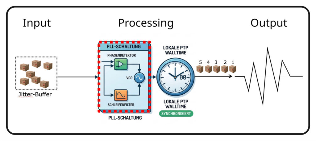
RTP and RTCP: Ordering the Chaos
Audio samples are encapsulated in RTP (Real-time Transport Protocol) packets, each carrying sequence numbers and timestamps. RTCP (RTP Control Protocol) ensures that every packet can be precisely associated with the PTP Wall Clock time. Since Layer-2 Ethernet has no inherent interest in delivery order, these packets frequently arrive "shuffled" at the receiver. A Jitter Buffer takes care of this: it holds incoming packets and plays them out in the correct sequence, clocked by the receiver's local oscillator — which is itself synchronised to the shared Wall Clock via PTP.

The PLL as a Flywheel

The PLL as a Flywheel Since network packet jitter (PDV) is always significantly higher than acceptable media clock jitter, the PLL (Phase-Locked Loop) in the receiver is critical. Think of it as a heavy flywheel: its rotational inertia keeps it running smoothly despite disturbances. A well-designed PLL responds only very sluggishly to fluctuations ("low corner frequency") and is not perturbed by every transient "twitch" in the network.

A "lightweight" flywheel that responded immediately to every network fluctuation would be a design failure.

The switch therefore makes no audible difference through the data it carries, but it does influence the quality of synchronisation by determining the degree of "calm" (low PDV) with which the PLL in the receiver can operate. A stable PTP network is thus the foundation for a low-jitter media clock.

IT System Architecture: A Comparison of Synchronisation Standards

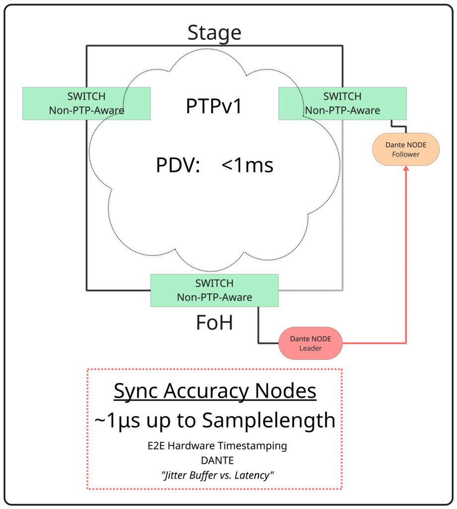
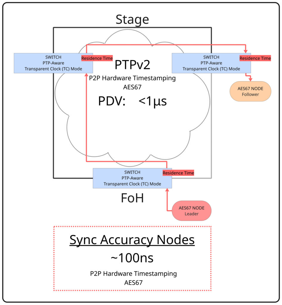
We now examine IT networks as transport media for various Audio-over-IP standards. Dante, developed by Audinate from 2006, targets a synchronisation accuracy of 1 µs between receivers (clock offset), with a guaranteed minimum of sample-accurate synchronisation. Given that PTPv2 was not defined until 2008, this is a creditable achievement, enabled by hardware timestamping in the Dante nodes.

A strict distinction must be drawn here: the synchronisation accuracy of Dante is 1 µs (in PTPv1 end-to-end mode). The physical packet jitter (PDV) on the network cable is often considerably higher.

In PTPv1, switches have no awareness of the protocol negotiated between the end devices (nodes) — they are "Non-PTP-Aware." This has the advantage of imposing no special requirements or costs on switch selection; even 100 Mbit/s switches and ports are not a disqualifying factor. The disadvantage, however, is that PDV in the network can reach up to 1 ms, which must be suppressed at the receiver through large jitter buffers and clock recovery.

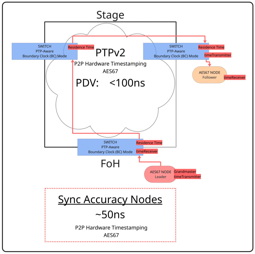
Only PTPv2 with Transparent Clocks (TC) in the switches reduces synchronisation deviations to below 100 nanoseconds, and with Boundary Clocks (BC) this can be optimised to below 50 nanoseconds.

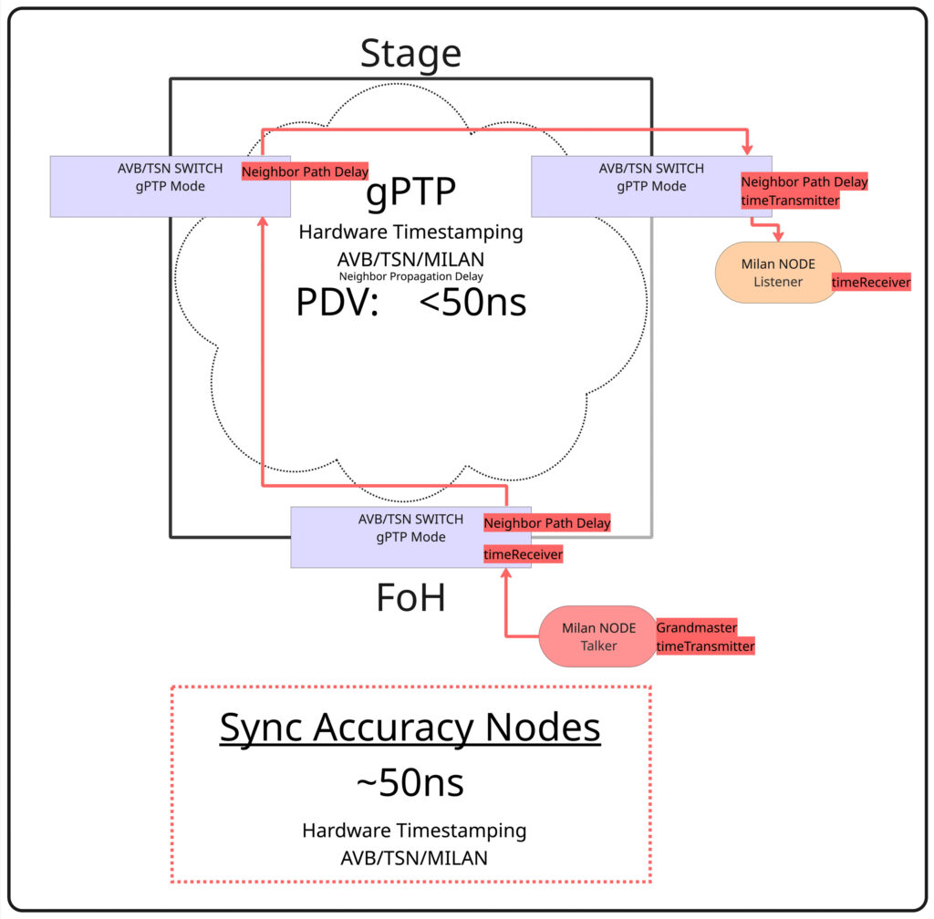
An AVB/TSN/Milan network achieves even lower PDV values. However, the synchronisation accuracy of Listeners to Talkers cannot be improved beyond what PTPv2 (BC) delivers for AES67, except under laboratory conditions.

It must be emphasised that all of the above refers to network synchronisation precision, not to media clock jitter. The network's packet jitter (PDV) is suppressed by jitter buffers at the receiver inputs and by clock recovery via the PLL. This is where the widely debated "clock sound differences" actually originate — not from the network packets themselves. Minimising packet jitter in IT networks through good design remains a worthwhile goal, as it reduces the burden on the jitter buffers and the PLL.

The Mathematics of Summation: The +6 dB Paradox

Let us briefly address something that borders on pedantry — but deliberately so.

We sum two coherent signals at 0 dBr each. What is the resulting level? 

+6 dB? Incorrect. 

The exact value is +6,0206dB!  [20 × log ₁₀(2) ≈ 6,0206 dB]

One might say, "don't be so fussy." But today, pedantry serves a purpose, so let us turn this around. If we round down to exactly 6.0000 dB, we must mathematically accept a phase offset of 7.89° at 20 kHz — which corresponds to exactly 1.09 µs. In that time, sound in air travels approximately 0.37 mm. This corresponds to the optimal synchronisation accuracy of Dante under ideal conditions — accuracy that can degrade, under adverse conditions such as high network load, Jumbo Frames, or 100 Mbit/s trunks, to as much as one full sample length.

Stress-Test

Next, let us subject a Dante PTPv1-based line array system to deliberate network jitter stress. In a purpose-built test system, it is possible to demonstrate a level error of 2 dB across the coverage area of a line array system (i.e. +4 dB instead of +6 dB summation). Assuming perfectly coherent signals at equal levels, this corresponds to a phase offset of 75° at 20 kHz — equivalent to approximately 10 µs of clock offset, or almost exactly one sample period at 96 kHz. This is precisely within the maximum Dante system specification.

Since clock recovery takes place in the receiver, and multiple receivers must be mutually synchronised, it makes sense to feed as many line array modules as possible from a single Audio-over-IP receiver with shared clock recovery — analogous to the way a single mixing console handles the task. In a self-powered (active) line array module with an onboard Dante card, this maximum error under poor PTPv1 conditions is exactly what is at stake — an error that can be reduced to the precision values above by adopting PTPv2 with Boundary Clocks. A system amplifier with an Audio-over-IP input feeding, for example, three line array modules provides identical clocking to all three modules even under worst-case network conditions. 

The 1-Sample Trap | From Legacy Interfaces to Audio-over-IP

Before system amplifiers were equipped with internal DSP processing, a central system controller handled all processing tasks for analogue amplifiers (amplifiers without DSP, regardless of topology — Class AB/D/H/TD, etc.). In such systems, there was only a single clock source, and the question of synchronising to a single Clock Leader was usually moot.

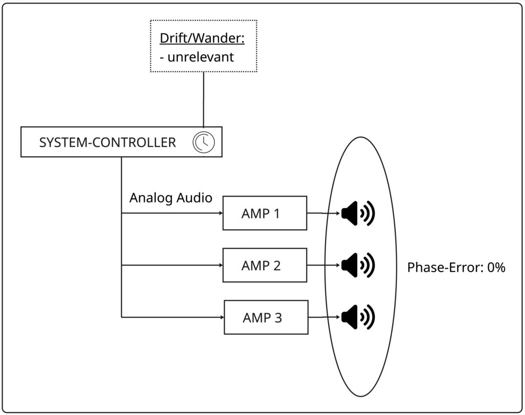
The next generation of system amplifiers was equipped with DSPs and could assume the processing role of the central controller. What happens when such a system is driven with analogue input signals?

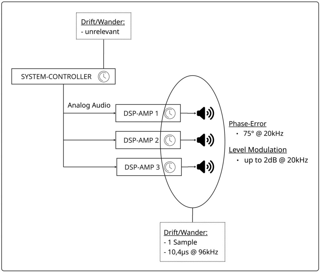
Each amplifier has a free-running clock. Assuming internal processing at 96 kHz and a drift of ±10 ppm against a perfect reference: Amplifier A's oscillator runs at 95,999.04 Hz, Amplifier B's at 96,000.96 Hz. After 1.04 seconds, the two amplifiers drift apart by exactly one sample (10.4 µs) — if one oscillator is perfect and the other carries maximum drift. In the worst case, where both oscillators drift in opposite directions, this interval halves accordingly. After approximately 28 hours, the total drift reaches one second — but there is no need for concern: the signal does not actually arrive one second later at one output than the other. In this real-time system, there is no absolute time reference. The maximum error is always bounded to one sample length (10.4 µs at 96 kHz); the "LFO rate" at which the error wanders within this window depends on oscillator precision.

Since the period of a 20 kHz signal is only 50 µs, a one-sample offset already produces a phase shift of up to 75° at 20 kHz. This error is exactly equivalent to the Dante PTPv1 worst-case scenario and produces the measured 2 dB level deviation at high frequencies. The system, protected by the analogue "guardrail," never reaches full cancellation (180° at 25 µs), but it permanently oscillates within a range that destabilises acoustic coupling. From this perspective, driving as many array modules as possible from a single amplifier is preferable — though this must be weighed against the power headroom and beam-steering requirements that necessitate individual drive per module.

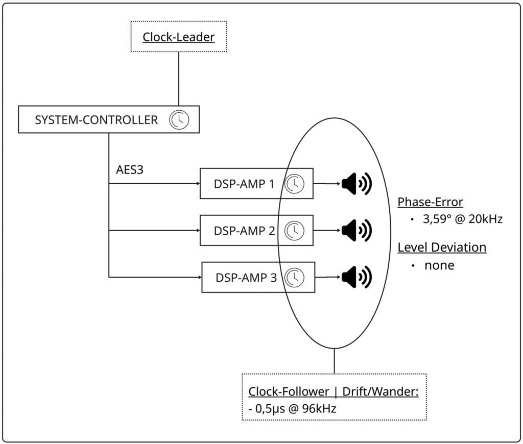
Analogue signal distribution protects against the total timing chaos of unsynchronised networks, but leaves systems trapped in the 1-Sample Trap. Only modern standards such as Milan or PTPv2 break this constraint, synchronising the converters so precisely that phase errors at 20 kHz become physically irrelevant. An instructive comparison is the digital classic AES3. The specification AES11-2009 (r2014) permits an input tolerance (jitter mask) of approximately 2.6% = ±270 ns (total jitter window of 540 ns) of the sample interval, equivalent to approximately 0.5 µs at 96 kHz. Summing our two coherent signals again yields +6.01633 dB instead of +6.0206 dB — a phase offset of 3.59° at 20 kHz. This is why the +6 dB pedantry was necessary. The internal PLL of the amplifiers filters this jitter and enables phase-locked playback. This value is the technological benchmark: a system using Milan or PTPv2 (BC) today delivers a clock signal that is already 5 to 10 times more precise at the input than the absolute limit of the classic AES3 interface.

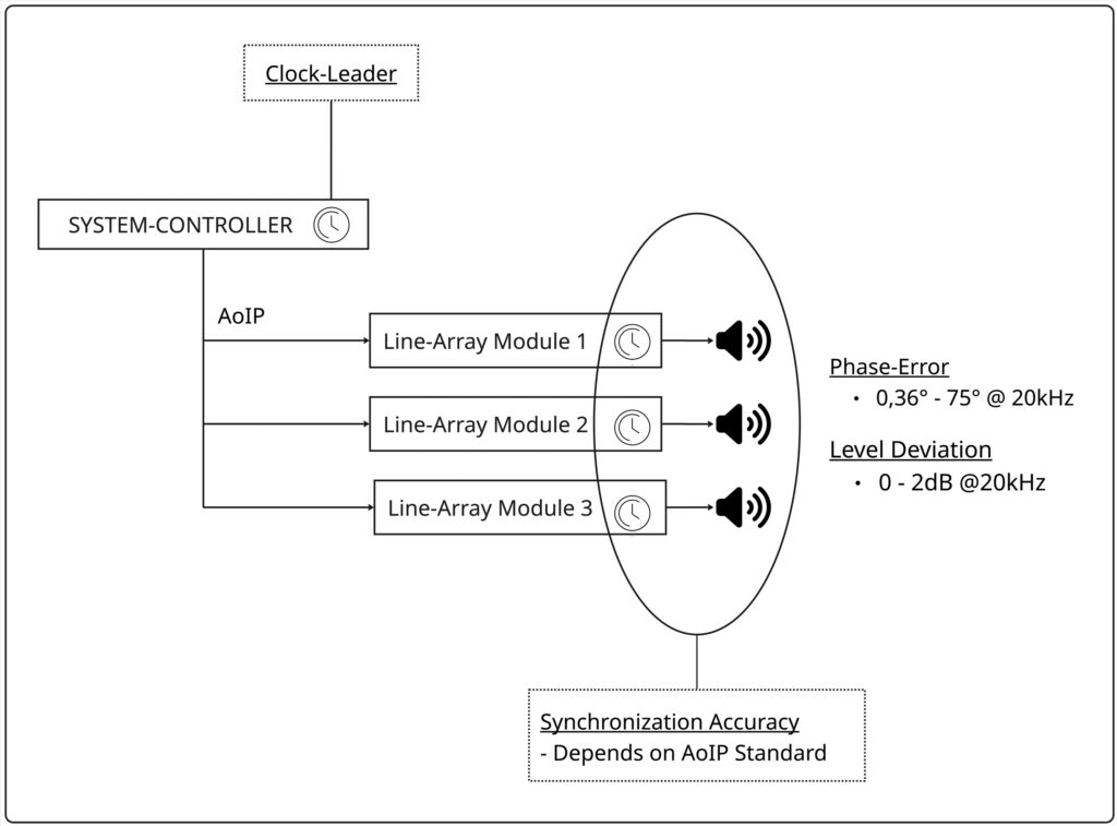
Next, we equip active self-powered line array modules with Audio-over-IP inputs. Synchronisation accuracy now depends on the AoIP standard in use, as well as the operating conditions — essentially: stressed or unstressed network?

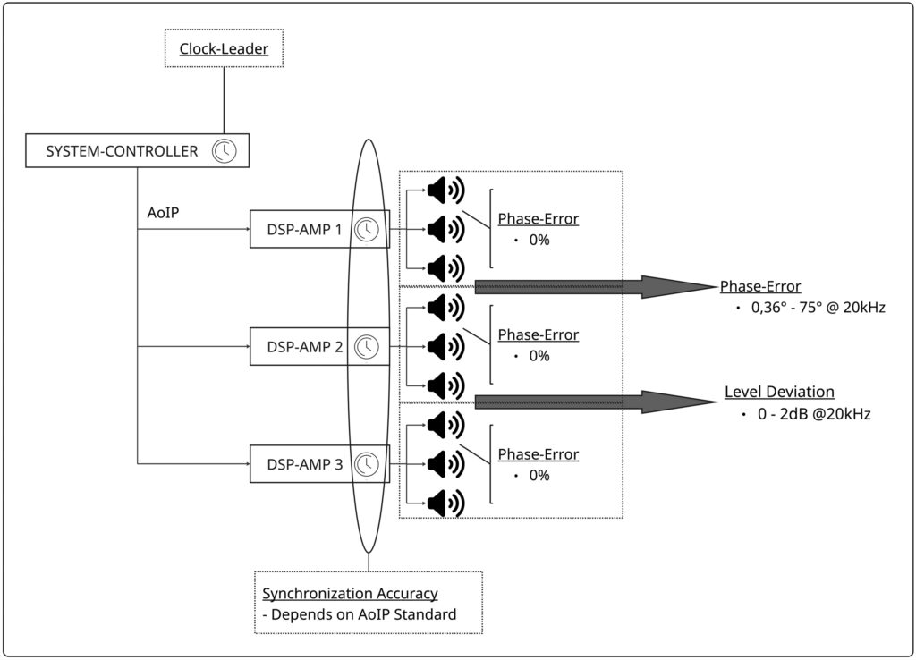
A further topology is to integrate AoIP inputs into the system amplifiers. In this case, phase errors and the resulting level modulation appear only at the module boundaries driven by the next amplifier.

Summary Table: PDV and Synchronisation Accuracy Across Audio System Scenarios

System Scenario	Jitter / PDV (Input)	Sync Accuracy (Node)	Total level @ 20 kHz	Acoustic Behaviour
AES3	~500 ns (0.5 µs)	< 20 ns (PLL)	6,02 dB	Phase-locked (reference)
AVB/TSN Milan (gPTP)	< 50 ns	~50 ns	6,02 dB	Absolutely coherent wavefront
AES67 (BC Mode)	< 100 ns	~50 ns	6,02 dB	Reference class (phase-locked)
AES67 (TC Mode)	< 1,000 ns (1 µs)	~100 ns	6,02 dB	Very stable
Dante (Best Case)	1,000,000 ns (1 ms)	~1,000 ns (1 µs)	6.00 dB	Industry standard
Dante (Worst Case)	1,000,000 ns (1 ms)	~10,420 ns (1 sample)	~4.01 dB	HF level reduction (static)
Analog-In (DSP)	n.a. (copper cable)	~10,420 ns (1 sample)	6,02 – 4,01 dB	HF level modulation (dynamic)

The ASRC Trap

In practice, differing sample rates must often be reconciled within the same system. This is where Sample Rate Converters (SRC) come into play. Synchronous SRCs pass the drift through rigidly; asynchronous converters (ASRCs) interpolate it continuously. Since they form a clock domain boundary, they must be positioned strictly at the edges of the system. If they are deployed multiple times in series within a line array segment, they induce uncontrollable latency offsets that simply destroy the acoustic coherence at high frequencies — the result of painstaking engineering effort. This is precisely why such configurations are avoided in practice: every array segment must be fed synchronously from a single clock domain, and the number of links is kept to a minimum to prevent interface jitter accumulation. System amplifiers that include SRCs in their AES3 inputs — which cannot be disabled via menu settings and are poorly documented in terms of their type (SRC vs. ASRC) — introduce additional error sources that degrade synchronisation accuracy.

Although modern ASRCs exhibit deterministic latency, they remain a clock domain boundary. Since each module in the array must independently estimate and regulate the ratio between its input and output clock, even tiny deviations in the tracking algorithms and filter group delays can lead to phase inconsistencies. In a system that depends on microsecond-level precision, this distributed clock recovery is an unnecessary risk. A system design that cascades ASRCs within media signal clusters is therefore the wrong approach. Sequential interpolation stages, each with their own filter artefacts and jitter transfer functions, smear the signal in time. Think of each ASRC as an independent "decision-maker" — but a line array system requires a single, system- wide "truth."

Summary:

Criteria for a Phase-Coherent Audio-over-IP System Design

Compared to PTPv1 with hardware timestamping in Dante modules (< 1 µs synchronisation accuracy), PTPv2 offers up to 10× greater precision with Transparent Clocks (< 100 ns) and up to 20× greater precision with Boundary Clocks (< 50 ns). To restate this clearly: Network Packet Jitter (PDV) ≠ Media Clock Jitter. Audio quality is determined by clock recovery in the receiver — this is the decisive parameter. In 2026, we do not need "miracle switches." We need clean system design: a precise Clock Leader, star- topology distribution, and the consistent elimination of free-running clocks or asynchronous sample rate converters within any line array segment. With these fundamentals in place, Audio-over-IP offers precision that is fully on a par with the mechanical construction of modern line arrays, and renders the drawbacks of interface-jitter-prone, daisy-chained AES3 wiring obsolete., AES3, Milan, AES67 (TC or BC), and Dante under best-case conditions are all equally capable of delivering precise audio signals to line array loudspeaker systems. Only Dante with PTPv1 under worst-case conditions falls into the same 1-Sample Trap as free-running DSP amplifiers driven by analogue inputs. The key distinction is that in the analogue case, the 75° phase error (2 dB level deviation) modulates dynamically and relatively quickly between the ideal +6 dB and the degraded +4 dB — whereas the error in Dante worst-case is comparatively static, and only arises when the receive cards are integrated directly into the line array modules themselves. Whoever wants to preserve the precision of a modern waveguide without squandering it at the electronic level must make converter synchronisation the highest priority.

Calculator:
PTP time, drift, jitter, sync, signal runtime in cables

Of course, the statements made here must also be mathematically plausible and comprehensible. Here you will find a calculator with which you can perform the following calculations:

• Convert UTC time to PTP time
• Convert PTP time to UTC time
• Calculate signal runtime over cable length
• Calculate clock drift, drift up to 1 sample and drift up to 1s difference, phase difference of clock drift at selectable frequency
• Calculate jitter in the nano- and microsecond range
• Calculate synchronization accuracy
• Conversion: Enter frequency and phase difference and calculate latency offset and sum level
• Conversion: Input total level of two coherent signals per 0dBr and calculate phase difference, as well as latency and sample offset
  

Excel Calculator - PTP time - Jitter - Signal-Propagation (EN)

1 file(s)

90KB

Buy with Paypal 5,99€

Want to go deeper?

Precision in the network is not a coincidence — it is the result of understanding your system. Anyone who knows why a line array loses coherence at 20 kHz can prevent it.

IT For AVs® – Networking for Event Technicians teaches the IT fundamentals that live event technicians actually need — in three days. And for those who want to go further: Mastering Event IT is coming as an additional module. One day, straight to the point: media networks and their IT requirements, PTP and synchronisation, routing fundamentals. Feeding internet into a venue and distributing it to specific disciplines — even on client networks where you never get near the router. Connecting a media server in the video VLAN with the lighting desk in the lighting VLAN. Thinking across disciplines, working across disciplines. IT For AVs® is currently taught in German. An English edition is in development.

if you want to be first to know when it launches, sign up below. No spam, no tricks. Just a signal when it matters.

→ I'm in:

List of sources

Perception & Psychoacoustics

[1]  E. Benjamin, B. Gannon (Dolby Laboratories): "Audibility of Jitter in Digital Audio Transmission"        AES Preprint 4826, 105th AES Convention, San Francisco, September 1998        https://www.aes.org/e-lib/browse.cfm?elib=8174

[2]  B. C. J. Moore: An Introduction to the Psychology of Hearing        6th Edition, Brill Academic Publishers, 2012. ISBN 978-9004252424 (Auditory threshold and temporal resolution)

Clock & Synchronization standards

[3]  IEEE: ‘IEEE Standard for a Precision Clock Synchronization Protocol for Networked Measurement and Control Systems – PTPv1’        IEEE Std 1588-2002        https://doi.org/10.1109/IEEESTD.2002.94144

[4]  IEEE: ‘IEEE Standard for a Precision Clock Synchronization Protocol for Networked Measurement and Control Systems – PTPv2’        IEEE Std 1588-2008        https://doi.org/10.1109/IEEESTD.2008.4579760

[5]  IEEE: ‘IEEE Standard for a Precision Clock Synchronization Protocol for Networked Measurement and Control Systems – PTPv2.1’        IEEE Std 1588-2019        https://doi.org/10.1109/IEEESTD.2020.9120376

[6]  BIPM / IERS: Coordinated Universal Time (UTC) and International Atomic Time (TAI)        Bureau International des Poids et Mesures        https://www.bipm.org/en/time-ftp/tai

[7]  U.S. Space Force: ‘IS-GPS-200: NAVSTAR GPS Space Segment/Navigation User Segment Interfaces’        GPS Interface Specification, current revision        https://www.gps.gov/technical/icwg/

Audio Interface & Digital Audio Standards

[8]  AES: ‘AES standard for digital audio – Serial transmission format for two-channel linearly represented digital audio data’        AES3-2009, Audio Engineering Society        https://www.aes.org/publications/standards/search.cfm?docID=2

[9]  AES: “AES recommended practice for digital audio – Synchronization of digital audio equipment in studio operations”        AES11-2009 (r2014), Audio Engineering Society        https://www.aes.org/publications/standards/search.cfm?docID=17

[10]  AES: AES standard for audio applications of networks – High-performance streaming audio-over-IP interoperability        AES67-2018, Audio Engineering Society        https://www.aes.org/publications/standards/search.cfm?docID=96

AVB / TSN / Milan

[11]  IEEE: IEEE Standard for Local and Metropolitan Area Networks – Timing and Synchronization for Time-Sensitive Applications (gPTP)        IEEE Std 802.1AS-2020        https://doi.org/10.1109/IEEESTD.2020.9121845

[12]  IEEE: ‘IEEE Standard for Local and Metropolitan Area Networks – Bridges and Bridged Networks (includes AVB/TSN)’        IEEE Std 802.1Q-2022        https://doi.org/10.1109/IEEESTD.2022.9870098

[13]  IEEE: IEEE Standard for Local and Metropolitan Area Networks – Forwarding and Queuing Enhancements for Time-Sensitive Streams (Credit-Based Shaper)        IEEE Std 802.1Qav-2009        https://doi.org/10.1109/IEEESTD.2010.5390974

[14]  IEEE: “IEEE Standard for Local and Metropolitan Area Networks – Enhancements for Scheduled Traffic (Time-Aware Shaper / TSN)”        IEEE Std 802.1Qbv-2015        https://doi.org/10.1109/IEEESTD.2016.7479742

[15]  AVNU Alliance: ‘Milan: A Pro AV Standard Based on AVB/TSN – Milan Specification’        AVNU Alliance / Milan Open Specification        https://www.milanspec.org

RTP / Network Transport

[16]  H. Schulzrinne, S. Casner, R. Frederick, V. Jacobson: ‘RTP: A Transport Protocol for Real-Time Applications’        IETF RFC 3550, July 2003        https://datatracker.ietf.org/doc/html/rfc3550

[17]  H. Schulzrinne, S. Casner: RTP Profile for Audio and Video Conferences with Minimal Control        IETF RFC 3551, July 2003        https://datatracker.ietf.org/doc/html/rfc3551

Dante / Audinate

[18]  Audinate Pty Ltd: Dante Audio Networking – Technical Overview and Whitepapers        Audinate, https://www.audinate.com/resources        https://www.audinate.com/resources        (Manufacturer reference – not an open standard)

CERN White Rabbit Project

[19]  M. Lipiński, T. Włostowski, J. Serrano, P. Alvarez: ‘White Rabbit: a PTP Application for Robust Sub-Nanosecond Synchronization’        ISPCS 2011, IEEE, September 2011        https://doi.org/10.1109/ISPCS.2011.6070148

Line array acoustics

[20]  M. Ureda: ‘Line arrays: Theory and Applications’        AES Preprint 5304, 110th AES Convention, Amsterdam, May 2001        https://www.aes.org/e-lib/browse.cfm?elib=9888

[21]  Gunness, D. and Tenney, W. Optimized Polar Patterns for Steerable Arrays        AES Preprint 6757, 121st AES Convention, San Francisco, 2006        https://www.aes.org/e-lib/browse.cfm?elib=13853        (Reference for waveguide tolerance and phase coherence in line arrays)